Regression Coefficient

REGRESSION

Description also available in video format (attached below), for better experience use your desktop.

Introduction

·     Regression analysis refers to assessing the relationship between the outcome variable and one or more variables. The outcome variable is known as the dependent or response variable and the risk elements, and co-founders are known as predictors or independent variables. The dependent variable is shown by “y” and independent variables are shown by “x” in regression analysis.

·   The sample of a correlation coefficient is estimated in the correlation analysis. It ranges between -1 and +1, denoted by r and quantifies the strength and direction of the linear association among two variables. The correlation among two variables can either be positive, i.e. a higher level of one variable is related to a higher level of another or negative, i.e. a higher level of one variable is related to a lower level of the other.

·  The sign of the coefficient of correlation shows the direction of the association. The magnitude of the coefficient shows the strength of the association.

·  For example, a correlation of r = 0.8 indicates a positive and strong association among two variables, while a correlation of r = -0.3 shows a negative and weak association. A correlation near to zero shows the non-existence of linear association among two continuous variables.

Least Square Method

·       The least square method is the process of finding the best-fitting curve or line of best fit for a set of data points by reducing the sum of the squares of the offsets (residual part) of the points from the curve. During the process of finding the relation between two variables, the trend of outcomes are estimated quantitatively. This process is termed as regression analysis. The method of curve fitting is an approach to regression analysis. This method of fitting equations which approximates the curves to given raw data is the least squares.

·       It is quite obvious that the fitting of curves for a particular data set are not always unique. Thus, it is required to find a curve having a minimal deviation from all the measured data points. This is known as the best-fitting curve and is found by using the least-squares method.

·        The least-squares method is a crucial statistical method that is practiced to find a regression line or a best-fit line for the given pattern. This method is described by an equation with specific parameters. The method of least squares is generously used in evaluation and regression. In regression analysis, this method is said to be a standard approach for the approximation of sets of equations having more equations than the number of unknowns.

·     The method of least squares actually defines the solution for the minimization of the sum of squares of deviations or the errors in the result of each equation.

·    The least-squares method is often applied in data fitting. The best fit result is assumed to reduce the sum of squared errors or residuals which are stated to be the differences between the observed or experimental value and corresponding fitted value given in the model.

·    There are two basic categories of least-squares problems:

• Ordinary or linear least squares
• Nonlinear least squares

·    These depend upon linearity or nonlinearity of the residuals. The linear problems are often seen in regression analysis in statistics. On the other hand, the non-linear problems are generally used in the iterative method of refinement in which the model is approximated to the linear one with each iteration.

Least Square Method Formula

Least-square method is the curve that best fits a set of observations with a minimum sum of squared residuals or errors. Let us assume that the given points of data are (x₁, y₁), (x₂, y₂), (x₃, y₃), …, (x_n, y_n) in which all x’s are independent variables, while all y’s are dependent ones. This method is used to find a linear line of the form y = mx + b, where y and x are variables, m is the slope, and b is the y-intercept. The formula to calculate slope m and the value of b is given by:

m = (n∑xy - ∑y∑x)/n∑x² - (∑x)²

b = (∑y - m∑x)/n

Here, n is the number of data points.

 

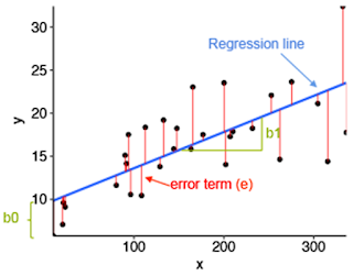
Least Square Method Graph

Look at the graph below, the straight line shows the potential relationship between the independent variable and the dependent variable. The ultimate goal of this method is to reduce this difference between the observed response and the response predicted by the regression line. Less residual means that the model fits better. The data points need to be minimized by the method of reducing residuals of each point from the line. There are vertical residuals and perpendicular residuals. Vertical is mostly used in polynomials and hyperplane problems while perpendicular is used in general as seen in the above image..

 

Method of Regression Coefficient

Regression coefficients can be defined as estimates of some unknown parameters to describe the relationship between a predictor variable and the corresponding response. In other words, regression coefficients are used to predict the value of an unknown variable using a known variable. Linear regression is used to quantify how a unit change in an independent variable causes an effect in the dependent variable by determining the equation of the best-fitted straight line. This process is known as regression analysis.

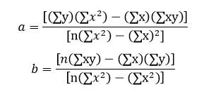
Formula for Regression Coefficients

The goal of linear regression is to find the equation of the straight line that best describes the relationship between two or more variables. For example, suppose a simple regression equation is given by y = 7x - 3, then 7 is the coeffiecient, x is the predictor and -3 is the constant term. Suppose the equation of the best-fitted line is given by Y = aX + b then, the regression coefficients formula is given as follows:

Here, n refers to the number of data points in the given data sets.

Regression Coefficients Graph

Properties of regression coefficient

1. The regression coefficient is denoted by b.

2. We express it in the form of an original unit of data.

3. The regression coefficient of y on x is denoted by b_yx. The regression coefficient of x on y is denoted by b_xy.

4. If one regression coefficient is greater than 1, then the other will be less than 1.

5. They are not independent of the change of scale. There will be change in the regression coefficient if x and y are multiplied by any constant.

6. AM of both regression coefficients is greater than or equal to the coefficient of correlation.

7. GM between the two regression coefficients is equal to the correlation coefficient.

8. If b_xy is positive, then b_yx is also positive and vice versa.

Video description

      Don’t forget to do these things if you get benefitted from this article

o   Visit our Let’s contribute page https://keedainformation.blogspot.com/p/lets-contribute.html

o   Follow our  page

o   Like & comment on our post